Charts Are Not Pictures

From Decoding Cost to Decision Leverage

Abstract

Most organizations treat charts as pictures — static outputs judged by aesthetics. This document treats them as capital allocation interfaces: systems that either free executive attention for decisions or consume it with decoding.

We introduce a structural scoring model — C×A×S (Channels × Arbitrariness × Simultaneity) — that ranks any visualization by expected cognitive cost, and four binary enforcement gates (G1–G4) that make “good chart” a testable condition rather than an opinion. A field audit of an operations dashboard redesign shows the model in practice: C×A×S dropped from 96 to 6, the decoding ratio fell from 0.60 to 0.13, and decisions per session doubled.

The argument proceeds in five steps: §1 defines the pipeline every chart passes through; §2 formalizes the decoding burden and its three drivers; §3 shows how interaction reduces cost without removing data; §4 identifies the structural violations AI introduces and the entropy curve they create; §5 measures the capital impact; §6 codifies the enforcement gates. Each section states a primary question so the document itself can be audited by the standard it proposes.

1. The Pipeline

Primary question: What is the minimum structure a chart must pass through to reach a decision?

TL;DR: Every chart is a pipeline: encoding → interaction → decision. Poor encoding inflates cognitive cost; interaction absorbs it.

Use §2 to score a chart (C×A×S), §6.1 to enforce gates (G1–G4), and §5.2 to justify redesign spend.

Every data visualization passes through four stages before it reaches a decision:

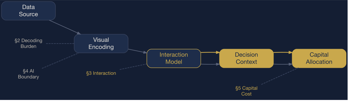
The visualization pipeline. Every distortion or optimization in this document maps to a specific stage.

The thesis: Visualization is not primarily decoration or discovery. It is a capital allocation interface — a system that either frees executive attention for decision-making or consumes it with decoding. Every encoding choice shifts cost between these two states.

Decoding Burden. The cognitive cost a reader pays to reverse-engineer a visual encoding before absorbing the message. Scales with channel count, encoding arbitrariness, and simultaneous density. Reduced by interaction, convention, and restraint.

Encoding Debt. Every visual channel added without a corresponding interaction path accumulates encoding debt — complexity the reader must repay on every glance.

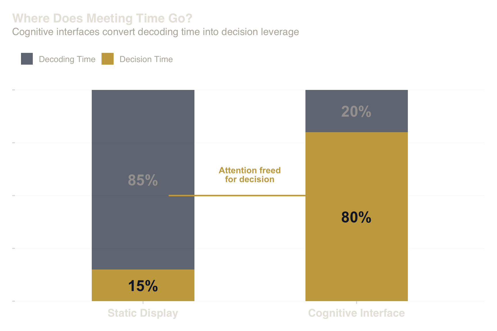
Gold = attention freed for decision. Grey = attention consumed by decoding.

2. The Decoding Burden

Primary question: What structural factors determine how hard a chart is to decode?

The pipeline’s second stage — visual encoding — is where cost accumulates. Every visual variable that is not self-explanatory adds a decoding step (Cleveland & McGill, 1984). Cost scales with distinct channels and mapping arbitrariness (Sweller, 1988). As a practical heuristic, treat >3 simultaneous encodings as a failure mode for general audiences (formalized as G2 in §4.3.1).

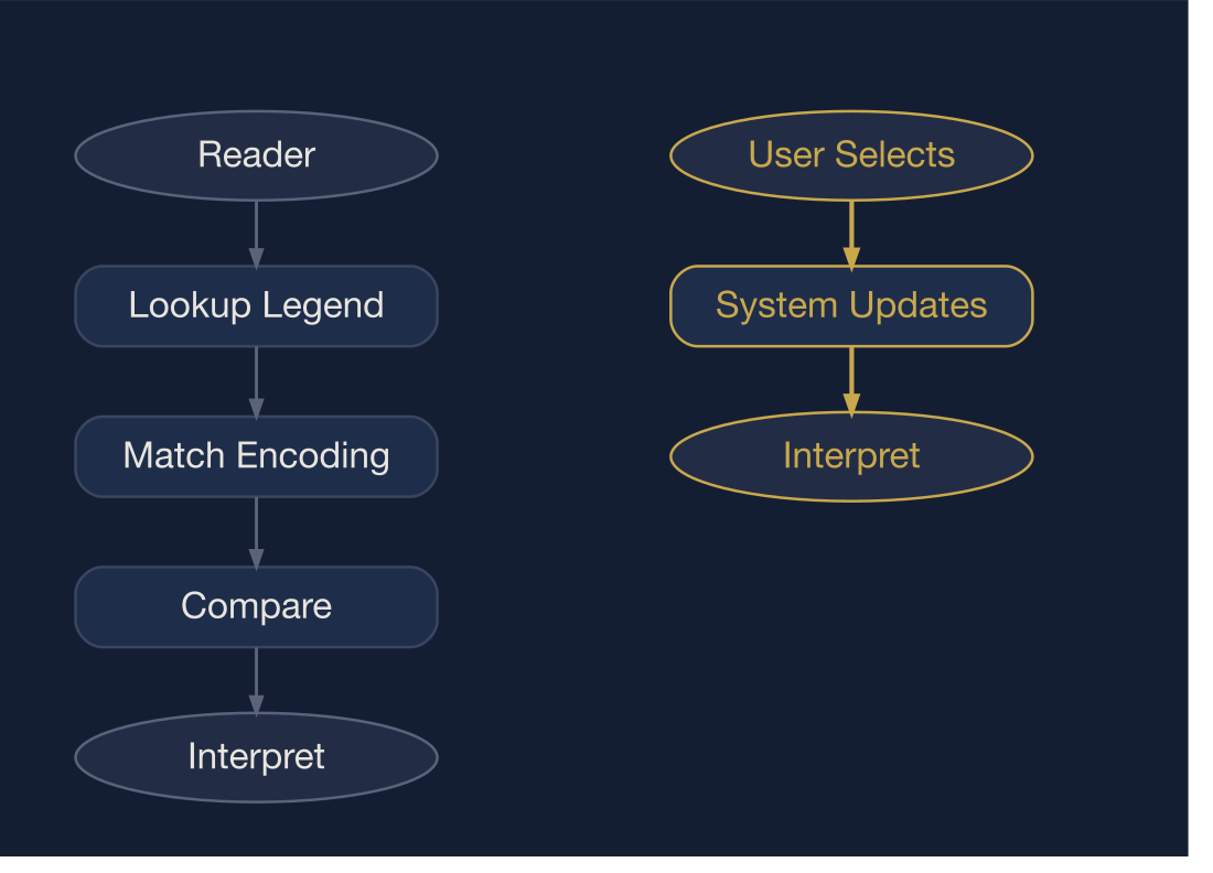
Static paths impose full cognitive cost on the reader. Interactive paths shift that cost to the system.

2.1 Formal Model

The decoding burden is a function of three structural drivers (two countable, one audience-relative):

\[ \text{Decoding burden} = C \times A \times S \]

(Also called “decoding cost” in some teams; this document uses “decoding burden” for the score.)

where:

Variable	Name	Measurement	Scale
\(C\)	Channels	Count of distinct visual encodings (position, size, shape, color, orientation, texture)	Integer ≥ 1
\(A\)	Arbitrariness	Encoding convention relative to audience. See scale below.	Ordinal 1–5
\(S\)	Simultaneity	Number of encodings required to answer the primary question without interaction	Integer ≥ 1

Operational test: \(S\) equals the number of distinct encodings the reader must hold simultaneously to answer the primary question in a single pass (no interaction).

Arbitrariness scale (A):

Value	Meaning	Examples
1	Universally conventional — no legend required	Sorted bars, position on axes, time → x-axis
2	Broadly conventional within professional context	Grouped bars, line charts with 2–3 series
3	Domain-conventional — known to specialists	Heatmap (for quants), forest plot (for epidemiologists)
4	Requires brief legend (1–3 items)	Custom color scale, size = variance
5	Custom mapping requiring legend + explanation	Bivariate choropleth, multi-hue stacked area

Counting rule for C: \(C\) counts only channels required to extract the primary question. Position, color, size, and shape each count if the reader must decode them. Threshold lines and direct labels typically do not count when they replace a legend lookup. Annotations count only if they introduce a new encoding the reader must decode (e.g., icon categories, color badges). For small multiples, count channels within one panel. Test: Does the reader need to decode this element to answer the primary question?

Why Multiplicative

Encoding costs amplify each other: high arbitrariness (\(A = 5\)) with high simultaneity (\(S = 3\)) forces the reader to hold 3 custom mappings simultaneously — a 15× burden, not 8×. One conventional channel (\(C=1, A=1, S=1\)) carries minimal cost. Addition would miss this nonlinearity. This is a structural model, not a psychometric one — useful for ranking designs, not predicting absolute task time.

Worked Example

Consider a bivariate choropleth map encoding unemployment (hue), inflation (saturation), and GDP growth (label size):

\[ C = 3, \quad A = 5 \text{ (bivariate color legend + size)}, \quad S = 3 \text{ (all needed for comparison)} \] \[ \text{Cost}_{\text{static}} = 3 \times 5 \times 3 = 45 \]

Add a hover-to-isolate interaction that reduces simultaneity to one channel at a time:

\[ S_{\text{interactive}} = 1, \quad \text{Cost}_{\text{interactive}} = 3 \times 5 \times 1 = 15 \]

Reduction: 67%. Interaction reduces simultaneity while holding channels constant — no data is removed, only the cognitive load per question.

Note: \(C\) is artifact-level (channels present); interaction mainly changes task-level requirement by collapsing \(S\).

Model Stress Test — Reviewer Disagreement

The C×A×S model requires a shared primary question to produce consistent scores. When reviewers disagree, the model exposes the ambiguity rather than hiding it.

Artifact: Executive dashboard showing quarterly revenue by region (bar chart) with YoY growth overlay (line) and target threshold (dashed line), color-coded by performance status (green/yellow/red).

Dimension	Reviewer A	Reviewer B	Disagreement source
Primary question	“Which regions missed target?”	“What is the YoY growth trend by region?”	Different questions → different scores
\(C\)	2 (position, color)	3 (position, color, line slope)	B counts the line overlay as a required channel
\(A\)	2 (traffic-light color is semi-conventional)	3 (YoY line requires legend to distinguish from bars)	B’s question makes the line encoding more central
\(S\)	2 (compare bar height to threshold)	4 (compare bars + read line + check color + reference threshold)	B’s question demands simultaneous decoding of more channels
Cost	8	36	4.5× difference

Arbitration rule: If the dashboard states a primary question, score to that question. If no stated question exists, it is a G1 violation — split the view. Log both scores; use the higher as the conservative estimate.

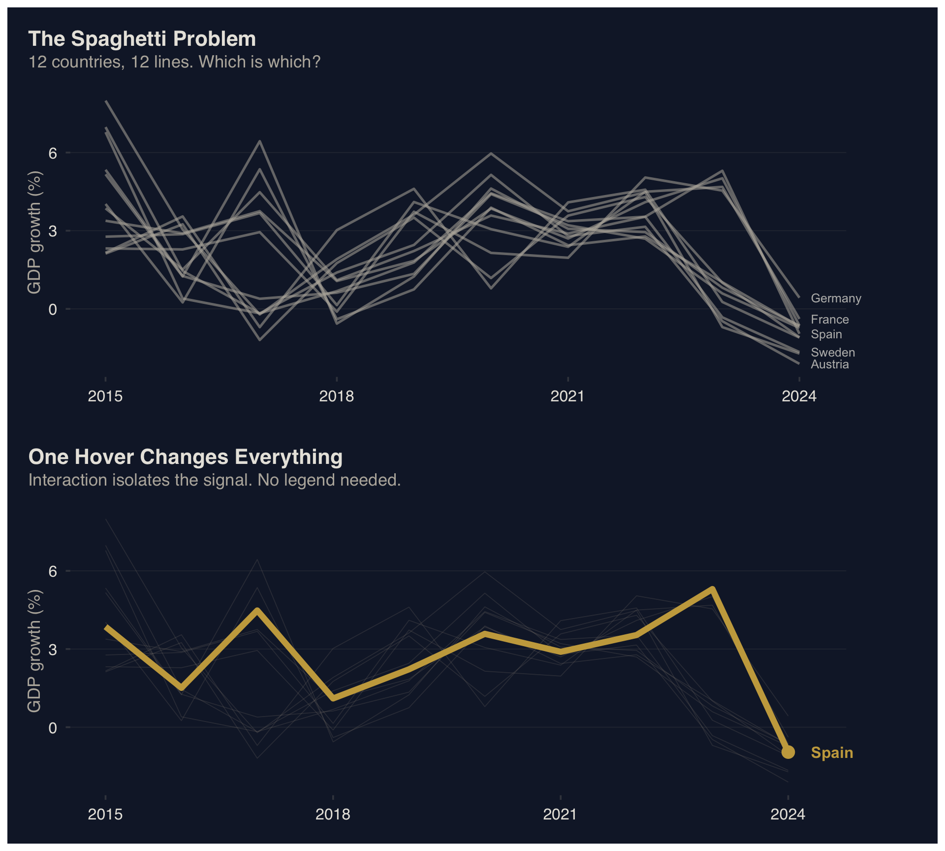
Top: 12 series competing for attention. Bottom: one hover isolates the signal; no legend lookup required.

Takeaway: Hover-to-highlight eliminates the legend lookup and isolates one series from twelve — reducing \(S\) from 12 to 1 without removing any data.

Output: a single integer score (C×A×S) plus a short note stating the assumed primary question and audience.

2.2 Case: Bivariate Map — The Simultaneity Cap

Three channels, three legend sections, three cognitive passes per country.

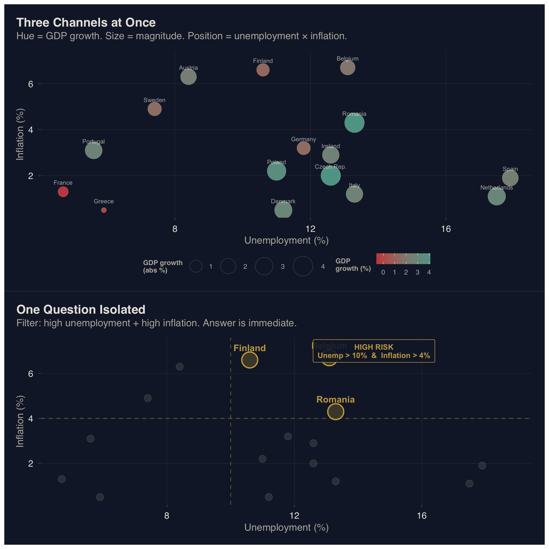
Top: three simultaneous channels force triple-pass decoding. Bottom: interaction isolates one question — high-risk countries.

Takeaway: Three simultaneous channels (\(C=3\), \(S=3\)) force triple-pass decoding. Filtering to one question collapses \(S\) to 1 — answer is immediate.

Dense encodings are not wrong — they are expensive. When \(A = 1\) (expert audience), higher \(S\) is tolerable. §6.2 formalizes the exceptions.

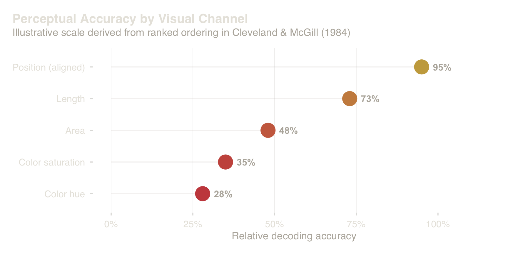
Position dominates; area and color force slower, less accurate decoding.

3. The Interaction Lever

Primary question: How does interaction reduce decoding burden without removing data?

The reduction lever for simultaneity (\(S\)) is interaction (Heer & Shneiderman, 2012). When the legend becomes a controller — hover, highlight, isolate, filter — the encoding collapses from many-to-many to one-to-one.

The structural levers are restraint (reduce \(C\)), convention (reduce \(A\)), and interaction (reduce \(S\)).

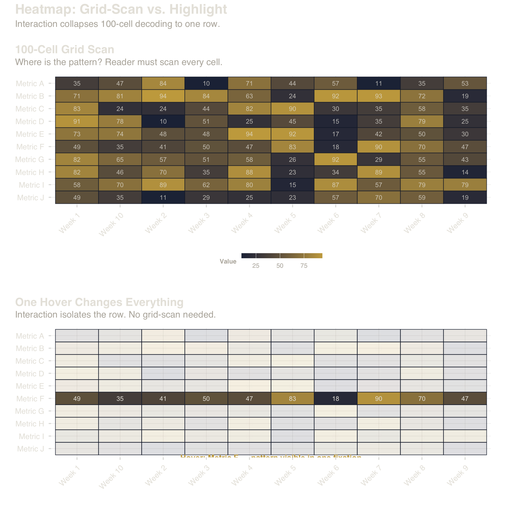
Top: a 10×10 heatmap forces grid-scanning across 100 cells. Bottom: one row highlighted — the reader sees the pattern in a single fixation.

Takeaway: A 100-cell grid forces serial scanning. Row highlight collapses the task to a single fixation — same data, fewer eye movements.

3.1 Cases: Heatmap and Multi-Series Hover

The pattern is consistent: interaction reduces \(S\) without removing data (\(C\) stays constant).

4. The AI Boundary

Primary question: What structural violations does AI introduce, and how does unchecked production velocity create organizational entropy?

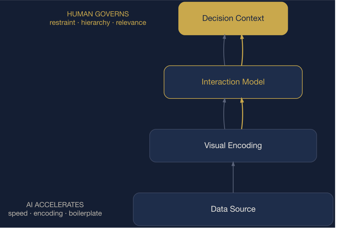
Data → Encoding → Interaction → Decision. AI accelerates the lower layers; human judgment governs the upper.

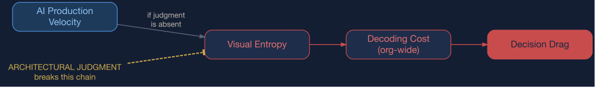
AI without architectural judgment amplifies decoding cost across the organization.

AI does not optimize structure — it cannot decide which views to build, what to omit, or how to protect hierarchy. The V1–V3 taxonomy below classifies how this gap manifests.

4.1 Structural Violation Taxonomy

AI-generated visualizations fail in recurring ways. Each violation maps to one variable in the decoding cost model (\(C \times A \times S\)):

Violation class	Model variable	Example
V1: Hierarchy failure	effective \(C\) (channels compete because visual weight is not allocated)	Every boxplot element at same visual weight
V2: Channel dominance	\(A\) (low-accuracy channel for primary comparison)	Stacked bar using color for primary comparison
V3: Legend dependency	\(S\) (simultaneity inflated by lookup requirement)	Scatter plot requiring legend for both color and shape

The three case studies below demonstrate each class in compact before/after form.

4.2 Case: V1 — Hierarchy Failure (Boxplot)

Violation V1: every element claims equal visual weight. Human judgment: remove noise, direct-label, make the median carry the hierarchy.

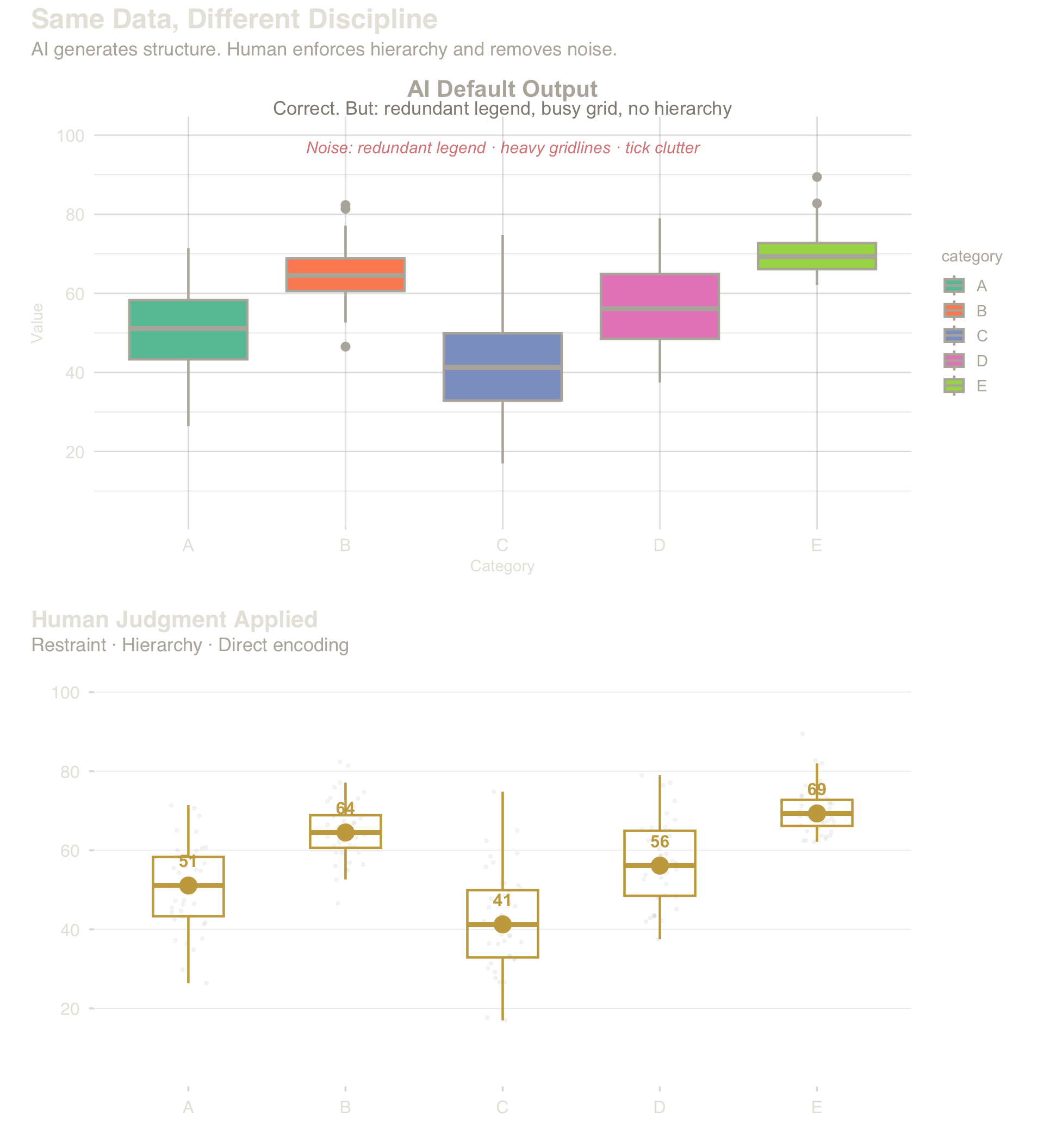
Top: AI default — correct structure, no visual hierarchy. Bottom: human judgment — restraint, direct labeling, deliberate ink.

Takeaway (V1): AI default: correct structure, zero hierarchy. Human edit: muted non-focus elements, direct labels, deliberate ink allocation. The data is identical — the difference is restraint.

4.3 Case: V2 — Channel Dominance (Bar Chart)

Violation V2: hue (lowest-accuracy channel) for the primary comparison instead of position (highest-accuracy). Redesign: sort by total, orient horizontally, label directly. Legend disappears.

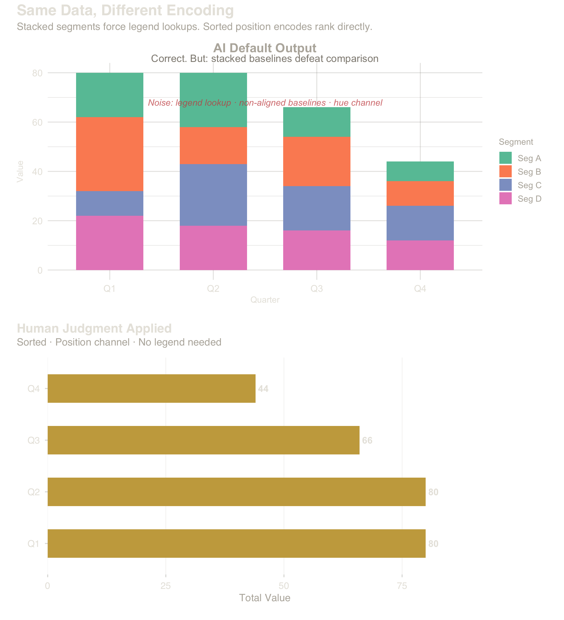
Top: stacked segments — hue channel, baseline shifts, legend required. Bottom: sorted horizontal bars — position channel, direct labels, no legend.

Takeaway (V2): Switching from hue (stacked bars + legend) to position (sorted bars + direct labels) eliminates the legend entirely. Channel choice is the design decision.

4.4 Case: V3 — Legend Dependency (Scatter Plot)

Violation V3: annotation is the legend, so a separate key inflates \(S\) with a redundant lookup. Alpha reduction, a single focal callout, and legend removal make the message immediate.

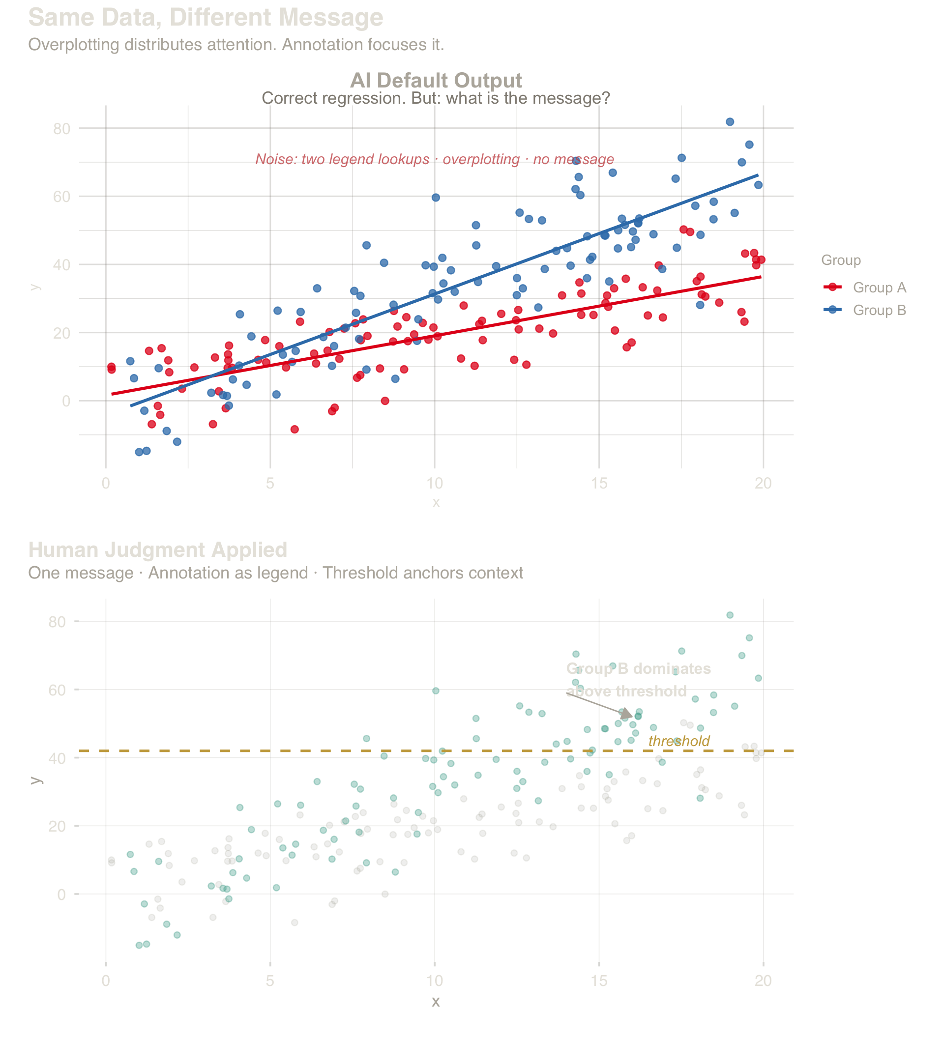
Top: two regression lines, legend, full overplotting. Bottom: alpha-reduced points, single annotated message, threshold line.

Takeaway (V3): When annotation carries the message, the legend becomes redundant. Removing it eliminates one full decoding step — from System 2 (lookup) to System 1 (read).

4.5 The Visualization Entropy Curve

As AI production velocity increases, visual artifacts grow faster than review capacity. The result is a divergence between output volume and structural quality.

Visualization Entropy Curve. The divergence between AI-driven output volume (convex growth) and organizational review capacity (concave saturation). When output exceeds review, unaudited artifacts accumulate — each carrying unpriced encoding debt.

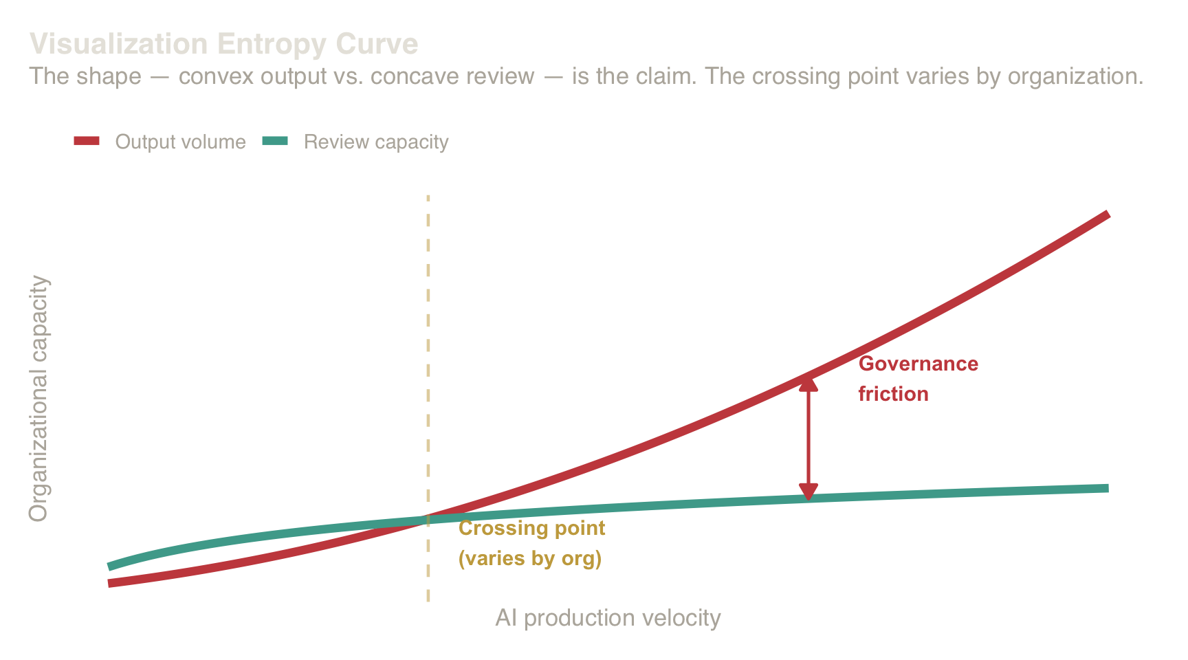
Without architectural judgment, artifacts accumulate faster than they can be reviewed.

The entropy gap is measurable:

\[ \text{Entropy Gap} = A_{\text{produced}} - A_{\text{reviewed}} \]

where A_produced = artifacts published per month and A_reviewed = artifacts passing G1–G4.

A widening gap requires either slowing production or scaling review capacity.

5. Measured Case, Capital Cost, and Gates

Primary question: How do we measure, price, and enforce decoding reduction?

5.1 Measured Case Study — Operations Dashboard Redesign

Context: A SaaS operations team used a weekly QBR dashboard with 8 KPIs (uptime, latency, error rate, support tickets, MAU, churn, NPS, revenue). The static version displayed all metrics simultaneously in a 2×4 grid. Each metric used 3–4 visual channels (line + color + threshold + annotation).

Before (Static Multi-KPI Dashboard):

• C×A×S score: \(C=4\), \(A=3\) (domain-conventional for ops team), \(S=8\) (all KPIs scanned per meeting) → Cost = 96
• Decoding ratio: 18 minutes decoding / 30 minutes total = 0.60
  
• Clarification questions: 12 per session (“What caused this spike?”, “Which threshold applies here?”, “Is this weekly or monthly?”)
  
• Decisions made (a committed action: escalate, allocate owner, change threshold, approve spend, defer with explicit next step): 2 per session (typically: escalate one issue, defer one investigation)

After (Interactive Single-Question Dashboard):

• Redesigned as tabbed interface: one primary KPI (uptime) on load, with tabs for drill-down into latency, errors, support. Each tab answers one question.
• Interaction: click tab → filtered view + relevant threshold line + automatic time window adjustment.
• C×A×S score: \(C=3\) (removed redundant color channel), \(A=2\) (simplified to universally conventional position + threshold), \(S=1\) (one KPI per view) → Cost = 6 (a 16:1 ratio reduction on the structural scale)

After — Measured outcomes (4-week average):

• Decoding ratio: 4 minutes decoding / 30 minutes total = 0.13 (78% reduction)
  
• Clarification questions: 2 per session (83% reduction)
  
• Decisions made: 4 per session (100% increase — freed attention reallocated to decision-making)

Capital cost avoided: Using the §5 method with 6 attendees × $500/hr × 14 minutes saved × 52 weeks = ~$200K/year.

Methodology note: Single-team before/after (n = 4 sessions each). Observer: product manager (non-presenting). Directionally consistent with C×A×S predictions but not a controlled experiment.

(A pharmaceutical DSMB redesign showed the same mechanism: Cost 75 → 4, decoding ratio 0.49 → 0.18, and decisions per session doubled.)

5.2 The Capital Cost of Decoding

The thesis lands here. Visualization is a capital allocation interface. When that interface has high decoding cost, executive attention — the organization’s scarcest resource — is consumed by legend lookups instead of strategic decisions.

You have probably sat in a meeting where this happens. A dashboard appears on screen and the room goes quiet — not because people are thinking, but because they are decoding. Someone asks “what does this axis mean?” Someone else traces a legend entry to a line. Twenty minutes later, the group has interpreted the chart but made no decision. The meeting runs over. The next one starts late. The decision gets deferred to email.

This is not merely a productivity problem. It is also an authority problem. Decoding shifts authority from decision-maker to chart-maker. Attention that should flow toward strategy flows instead toward comprehension.

The cost is measurable:

5.2.1 Structural Comparison: QBR with Static vs. Interactive Views

Metric	Static dashboard	Cognitive interface	Delta
Executive committee time	40 min	40 min	—
Time decoding (“what does this axis mean?”)	25 min (63%)	5 min (13%)	−20 min
Time deciding (capital allocation, hiring, strategy)	15 min (37%)	35 min (87%)	+20 min
Decisions per session	1	3–4	×3

The cost model is conservative: it counts only executive time in a single meeting cadence.

5.2.2 Sensitivity Analysis — Annual Cost of Decoding Burden

Scenario	Attendees	Rate ($/hr)	Min saved	Cadence	Annual cost avoided
Conservative	4	$250	5	Monthly (12×)	$1,000
Typical — small team	6	$400	10	Bi-weekly (26×)	$10,400
Typical — exec QBR	6	$500	20	Weekly (48×)	$96,000
High-frequency ops	8	$600	15	Weekly (48×)	$115,200
C-suite strategic	10	$1000	30	Monthly (12×)	$60,000

Formula: annual_cost = attendees × rate × (minutes_saved / 60) × sessions_per_year

Even the conservative scenario ($1K/year) exceeds the cost of a single dashboard redesign sprint. The typical exec QBR scenario ($96K/year) represents 1.2 FTE analyst salaries — capital currently consumed by decoding instead of analysis.

The capital efficiency rule: if decoding_minutes / total_minutes > 0.3, the visualization pipeline (§1) has a structural defect. The fix is upstream — encoding and interaction, not presentation polish.

5.2.3 How to Measure It

Assign one observer to your next QBR. Every time someone asks “what does this mean?”, looks up a legend, or re-reads an axis — that is a decoding event. Sum the time. Divide by total meeting time. If the ratio exceeds 0.3, the encoding has a structural defect. If it exceeds 0.5, the meeting is a decoding session, not a decision session.

6. Principles and Enforcement Gates

Primary question: What rules make “good chart” a testable condition?

Three things hold across tools and audiences:

1. Performance. Slow interaction is no interaction. Responsiveness is part of the design (Card, Moran & Newell, 1983; Norman, 1988).
2. Interaction. When the legend controls the view, cognitive load drops. Hover → highlight → isolate generalizes across chart types (Heer & Shneiderman, 2012).
3. Restraint. Fewer channels, clearer hierarchy, deliberate choice of what not to show. Tufte’s (1983) data-ink ratio operationalizes restraint; Wilkinson’s (2005) grammar of graphics provides the formal vocabulary.

Reviewer checklist (one pass): stated primary question (G1); answerable without >3 channels at once (G2); primary read requires ≤1 legend lookup (G3); interactions feel instantaneous (<200 ms) or the view degrades cleanly to static (G4).

6.1 Enforcement Gates

The principles above crystallize into four binary gates. Each is operationally testable in review — a visualization that fails any gate carries encoding debt and must be redesigned before shipping:

Here, “channel” means a visual encoding required for the primary question (position, size, color, shape, etc.).

Gate	Condition	Action
G1	questions_per_screen > 1	→ Split or layer. One question per view.
G2	channels_per_fixation > 3	→ Remove channels or add interaction to reduce \(S\).
G3	legend_lookups_per_view > 1 for the primary question	→ Redesign encoding. Prefer direct labels/annotation so the primary read is legend-free.
G4	interaction_latency_ms > 200	→ Optimize or degrade gracefully to static. >200 ms breaks perceived direct manipulation (Card, Moran & Newell, 1983).

These gates are binary — a chart either passes or it does not. Ambiguity about quality is reduced when failure can be tied to a specific condition.

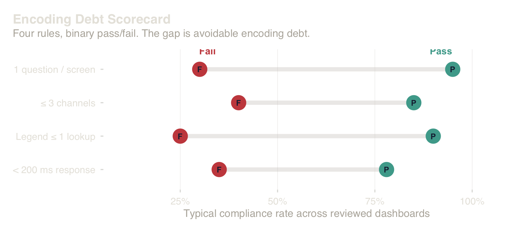
Four testable rules. Pass = green. Fail = encoding debt.

6.2 When Static Density Is Appropriate

The model does not prescribe interaction universally — it prescribes reducing \(S\). Two exceptions apply. Expert audiences with conventional encoding (\(A = 1\)) tolerate higher simultaneity because the mapping is already internalized; radiologists reading MRI sequences and quants reading heatmaps do not need legends. Print and archival media cannot support interaction; small multiples, direct labeling, and aggressive channel reduction achieve the same \(S\)-reduction without interactivity. In both cases, the gate that changes is different (G2 threshold relaxes for experts; G4 does not apply for print), but the cost model still applies.

References

• Cleveland, W. S., & McGill, R. (1984). Graphical Perception: Theory, Experimentation, and Application to the Development of Graphical Methods. Journal of the American Statistical Association, 79(387), 531–554.
• Kahneman, D. (2011). Thinking, Fast and Slow. Farrar, Straus and Giroux.
• Tufte, E. R. (1983). The Visual Display of Quantitative Information. Graphics Press.
• Bertin, J. (1967/1983). Sémiologie Graphique. English edition: Semiology of Graphics. University of Wisconsin Press.
• Munzner, T. (2014). Visualization Analysis and Design. CRC Press.
• Heer, J., & Shneiderman, B. (2012). Interactive Dynamics for Visual Analysis. Communications of the ACM, 55(4), 45–54.
• Shneiderman, B. (1996). The Eyes Have It: A Task by Data Type Taxonomy for Information Visualizations. IEEE Symposium on Visual Languages, 336–343.
• Card, S. K., Moran, T. P., & Newell, A. (1983). The Psychology of Human-Computer Interaction. Lawrence Erlbaum Associates.
• Norman, D. A. (1988). The Design of Everyday Things. Basic Books.
• Few, S. (2006). Information Dashboard Design. O’Reilly Media.
• Wilkinson, L. (2005). The Grammar of Graphics (2nd ed.). Springer.

Generated with R 4.5.1 · marcelokatogui.com