CV vs Proper Validation

Why Cross-Validation Can Still Mislead You

1. The Premise

You train a model. You run 5-fold cross-validation. The RMSE looks great. You deploy.

In production, the model performs significantly worse than the CV estimate suggested.

“But I cross-validated!”

The problem is not the model. The problem is what the evaluation is targeting.

Cross-validation estimates the expected prediction error under the resampled data-generating process — the mechanism implied by randomly shuffling and re-splitting rows (Arlot & Celisse, 2010). Formally, CV targets:

\[ \widehat{\mathcal{R}}_{CV} = \frac{1}{K} \sum_{k=1}^{K} \widehat{R}_k \]

where \(\widehat{R}_k\) is the loss on the \(k\)-th held-out fold. The deployment risk, by contrast, is:

\[ \mathcal{R}_{deploy} = \mathbb{E}_{(x,y) \sim P_{future}} \left[ L(f(x), y) \right] \]

When \(P_{future} = P_{train}\) (the data are exchangeable), \(\widehat{\mathcal{R}}_{CV}\) is a consistent estimator of \(\mathcal{R}_{deploy}\). When they differ, the optimism bias (Hastie et al., 2009, Ch. 7) is:

\[ \text{Bias} = \mathbb{E}[\widehat{\mathcal{R}}_{CV}] - \mathcal{R}_{deploy} \]

This bias is negative (i.e., CV underestimates deployment error) whenever the resampled distribution \(P_{mix}\) is more favorable than \(P_{future}\). The sign reverses if deployment conditions happen to be easier than the training mixture, though this is atypical.

For the reshuffled estimate to equal the deployment estimate, the observations must be exchangeable — any permutation of \((x_1, y_1), \ldots, (x_n, y_n)\) must have the same joint distribution. This is the exchangeability assumption — a condition satisfied by IID data, but also by broader classes of distributions. Exchangeability is sufficient for CV consistency; strict independence is not required.

Two common data structures break exchangeability:

1. Time-dependent data — the data-generating process changes over time. Random CV estimates risk under the mixture distribution \(P_{mix} = \frac{1}{n}\sum_{t=1}^n P_t\), while deployment uses \(P_{future}\). Under drift, \(P_{mix} \neq P_{future}\).
2. Clustered data — observations within a group share latent variables \(\alpha_g\). Random CV conditions on partial realizations of \(\alpha_g\) from same-group training rows, shrinking the apparent predictive variance below its true deployment-level value.

When exchangeability fails, random CV admits structure into the evaluation that will not exist at deployment. The result: an optimistic error estimate that reflects the reshuffled distribution \(P_{mix}\), not the deployment distribution \(P_{future}\).

This document demonstrates both failure modes with reproducible simulations, quantifies the optimism bias, and shows the correct alternative for each.

Deployment Scenarios

Before interpreting any validation result, define the deployment scenario precisely:

Question	Deployment Target	Required Split
Predict future time for the same population?	\(P_{future}\)	Time-blocked
Predict a new individual never seen before?	New \(\alpha_i\)	Group-blocked
Predict a new time for an existing individual?	\(P_{future} \mid \alpha_i\) known	Group-aware time-blocked
Predict same population, same time?	\(P_{train}\)	Random CV is valid

The correct split strategy follows directly from the deployment target. Mismatching the two is the root cause of optimism bias.

2. Time-Dependent Regime Shift

The Setup

Consider a system observed over 2,000 time steps. For the first half (\(t \leq 1000\)), the response \(y\) increases with \(x\). After \(t = 1000\), the relationship reverses — \(y\) now decreases with \(x\):

\[ y_t = \begin{cases} 2x_t + \varepsilon_t & \text{if } t \leq 1000 \\ -2x_t + \varepsilon_t & \text{if } t > 1000 \end{cases} \]

\[ \varepsilon_t \sim \mathcal{N}(0, 1) \]

This is a regime shift — a structural break where the underlying data-generating process changes discontinuously. In practice, this arises from policy changes, market corrections, behavioral shifts, or any non-stationary process. The coefficient flips from \(+2\) to \(-2\): not a subtle drift, but a complete reversal.

Random 5-Fold CV

Standard cross-validation shuffles all 2,000 observations randomly across 5 folds (Bergmeir & Benítez, 2012). This destroys the temporal order. Each fold now contains a mixture of pre- and post-break data — roughly 500 observations from Regime 1 and 500 from Regime 2.

The consequence: when the model trains on 4 folds, it has already seen future data. And when it validates on the held-out fold, that fold contains past data the model was built from. The test and training distributions overlap, sharing data from both regimes in every split.

Proper Time-Blocked Split

The correct approach respects the arrow of time: train only on the past (\(t \leq 1000\)), then evaluate on the future (\(t > 1000\)). The model never sees data from the regime it will be tested on.

This is what deployment looks like — you build a model today and apply it tomorrow. If the world changes between now and then, only a time-blocked evaluation will reveal it.

The Gap

The bar chart below compares the two RMSE estimates. The left bar is what random CV reported; the right bar is what actually happens when the model faces unseen future data.

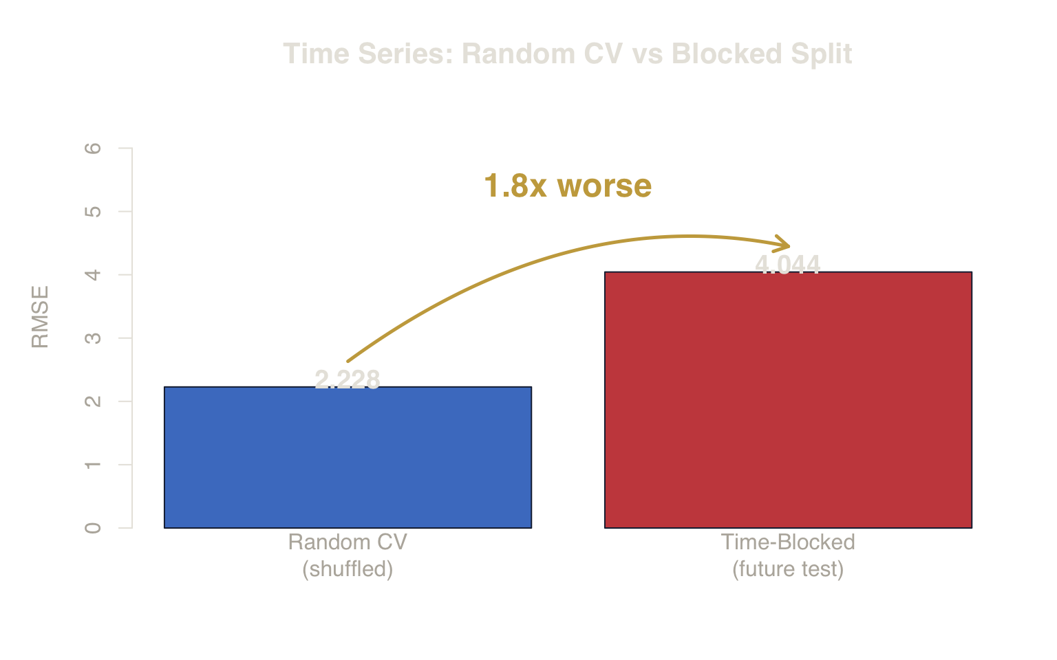
Figure 1. Optimism Bias in Time Series. Random CV underestimates the true deployment error by mixing past and future data, failing to detect the regime shift.

Random CV RMSE: 2.228 ± 0.023 — looks acceptable.

Time-Blocked RMSE: 4.044 — the true out-of-sample error.

Random CV underestimates the real error by a factor of 1.8x.

Deployment Insight

If your data has temporal structure, random shuffling lets the model “peek” into the future. A model that looks great in cross-validation may fail completely when it faces a future regime it wasn’t tested on.

Visualizing the Regime Shift

The scatter plot below shows all 2,000 observations colored by regime. The gold dashed line at \(t = 1000\) marks the structural break. Notice how the cloud of points mirrors across the break — the same predictor \(x\) drives opposite responses. A linear model trained on both regimes converges to the average coefficient under \(P_{mix}\): under equal regime sizes and homoskedastic noise, \(\hat{\beta} \approx \frac{1}{n}\sum \beta(t) \approx 0\). The model is consistent for \(P_{mix}\) but misaligned with \(P_{future}\), where \(\beta = -2\). Random CV evaluates under that same favorable mixture; time-blocked evaluation exposes the mismatch.

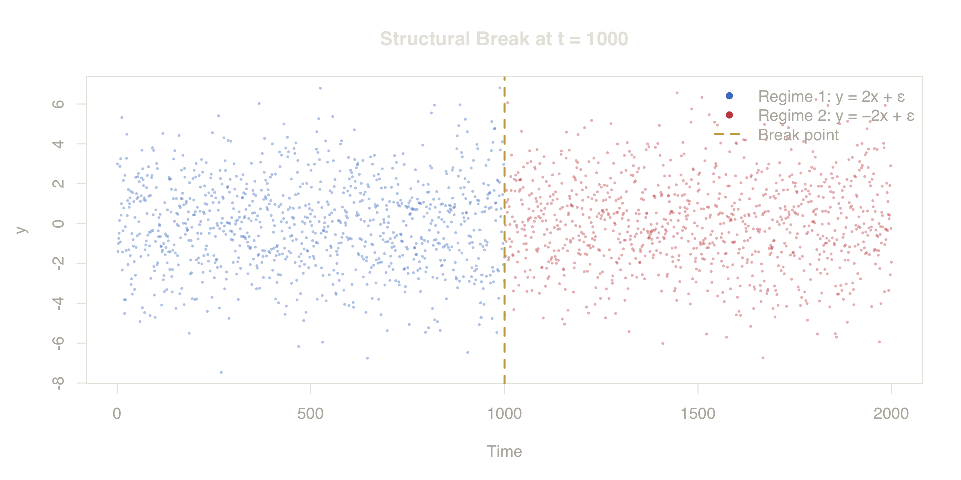
Figure 2. Visualizing the Structural Break. The relationship between X and Y completely reverses at t=1000. Random CV evaluates on a mixture of both, masking the failure.

Fold-Level Error Distribution

Point RMSE estimates hide the variance across folds. The boxplot below shows per-fold RMSE for random CV. Notice the narrow spread — all folds see the same mixture of regimes, so each fold’s error is similarly biased. The time-blocked estimate (red dashed line) sits far above the fold distribution, confirming that the optimism is structural, not a single-fold anomaly.

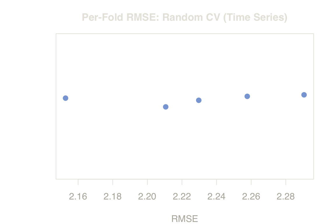
Figure 3. Variance Across Folds. Random CV’s RMSE remains tightly clustered and optimistic. The red dashed line (Blocked Split) shows the true error encountered at deployment.

2b. Gradual Coefficient Drift

The regime-flip above is pedagogically clear but extreme. Real-world non-stationarity is usually subtler — a slow drift rather than a discontinuity. To verify that CV bias is not an artifact of the extreme scenario, we simulate linear coefficient decay:

\[ \beta(t) = 2 - 1.5 \cdot \frac{t}{n}, \qquad y_t = \beta(t)\, x_t + \varepsilon_t \]

The slope starts at \(2\) and decays to \(0.5\) — a gradual weakening, not a sign reversal. If random CV is still optimistic under this smooth drift, the problem is not about catastrophic breaks; it is about any violation of stationarity.

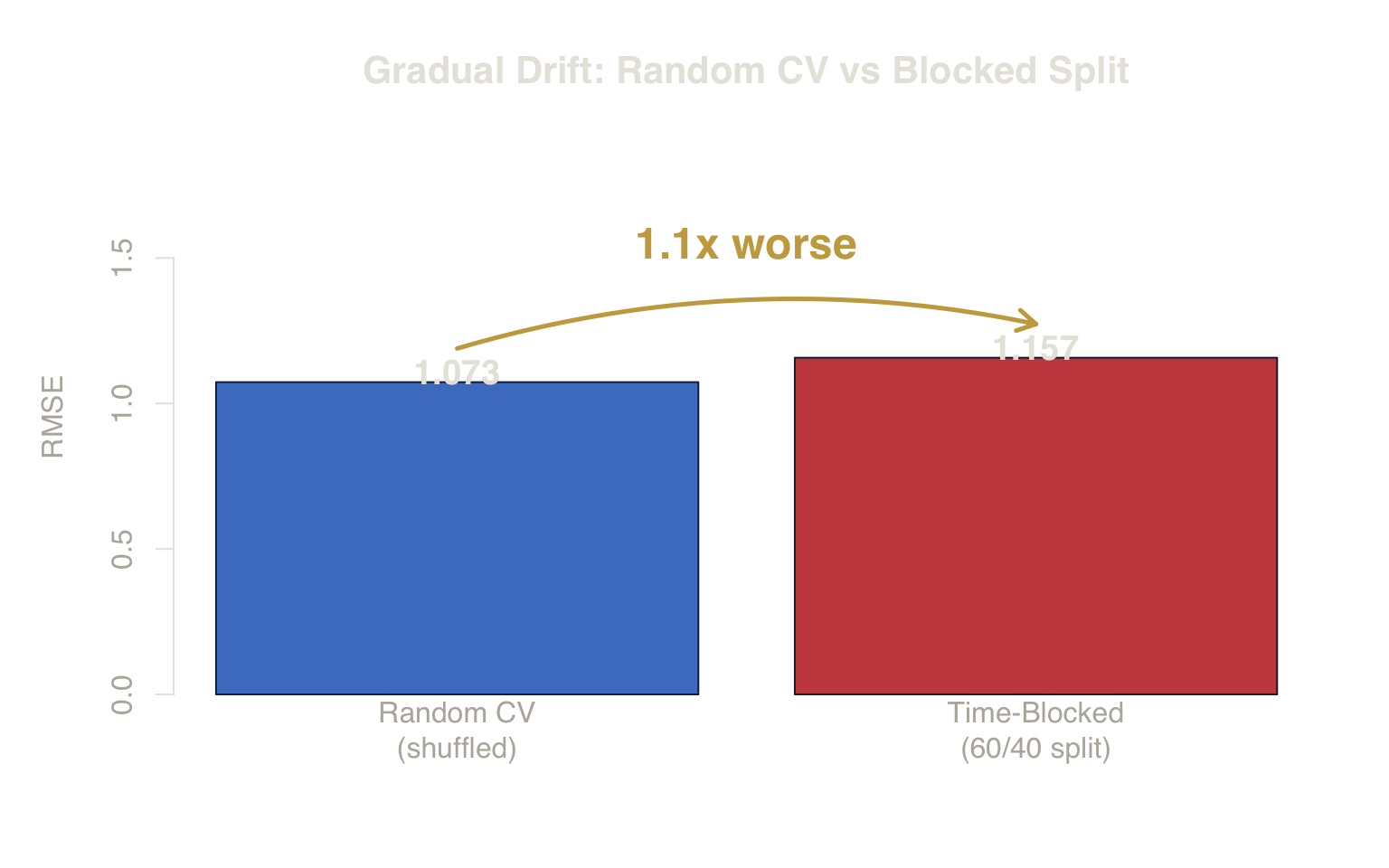
Figure 4. Impact of Gradual Drift. Even without a catastrophic regime flip, random CV fails to account for the slow degradation of predictive quality over time.

Even with smooth, moderate drift, random CV remains optimistic. The gap is smaller than the regime-flip scenario — confirming that severity scales with the magnitude of non-stationarity — but the direction of bias is the same. Random CV averages across time, masking horizon-specific degradation.

Deployment Insight

For time-dependent data, do not trust a single summary statistic from shuffled CV. Evaluation must test your model exactly as it will be used: on data that occurs after the training window has closed.

2c. Walk-Forward Validation

A single time-blocked split (train on [1, \(t\)], test on [\(t\)+1, \(n\)]) depends on the choice of split point. Walk-forward validation (also called expanding-window or rolling-origin evaluation; Tashman, 2000) removes this dependency by testing on a sequence of future windows:

1. Train on \([1, t_0]\), test on \([t_0+1, t_0+h]\)
2. Train on \([1, t_0+h]\), test on \([t_0+h+1, t_0+2h]\)
3. Continue until the end of the series.

Each step trains only on the past and evaluates on genuinely unseen future data. The resulting RMSE trajectory shows how performance degrades as the deployment horizon extends.

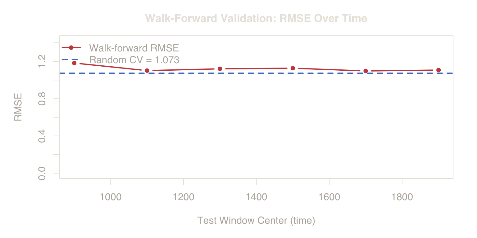
Figure 5. Performance Decay. As the test period moves further from the training window, RMSE rises. Shuffled CV (blue line) is blind to this decay because it averages across all time origins.

The walk-forward trajectory rises as the test window moves further from the training period. Random CV (blue dashed line) sits at the bottom, averaged across all time, blind to this degradation.

Deployment Insight

Walk-forward validation acts as a stress test. It doesn’t just give you a better RMSE; it tells you your model’s “shelf life” by showing how quickly accuracy degrades as the future moves further from the training data.

Walk-forward validation serves two purposes: it provides a more honest RMSE estimate, and it diagnoses drift by revealing how error changes across the deployment horizon. The slope of the RMSE trajectory directly quantifies the rate at which the model’s assumptions diverge from reality.

Note that the expanding training window introduces a competing effect: more training data generally reduces estimation variance. The fact that RMSE nevertheless rises confirms that bias from coefficient mismatch dominates the variance reduction from additional observations.

3. Clustered Data Leakage

The Setup

Now consider a different violation. We have 200 customers, each observed 10 times. Each customer has two properties:

1. Observable features (\(f_1\), \(f_2\)) — customer-level characteristics visible to the model (e.g., age, tenure). These are constant across all 10 rows for the same customer.
2. An unobserved random intercept \(\alpha_i\) — a customer-specific baseline that shifts all outcomes up or down. This is not in the feature set.

\[ y_{ij} = 5 + \alpha_i + 0.5\, f_{1i} + 0.3\, f_{2i} + 2\, x_{ij} + \varepsilon_{ij} \] \[ \alpha_i \sim \mathcal{N}(0, 3), \quad \varepsilon_{ij} \sim \mathcal{N}(0, 1) \]

The critical ratio: \(\sigma_\alpha = 3\) is three times larger than \(\sigma_\varepsilon = 1\). Most of the variation in \(y\) is between customers, not within them. And because \(\alpha_i\) is not a feature, the model must infer it indirectly — from the patterns in nearby rows.

We use a K-nearest-neighbors (KNN) regressor rather than a linear model. Why? A linear model fits global coefficients — it cannot exploit the fact that same-customer rows share an intercept, regardless of how you split the data. KNN, by contrast, predicts each row from its nearest neighbors. When same-customer rows leak into training, they become exact matches on the customer-level features (\(f_1\), \(f_2\)) — and they carry the shared \(\alpha_i\) directly into the prediction. This is the mechanism that makes the leakage visible.

Random CV (Leaks Customers)

Random 5-fold CV assigns rows to folds ignoring customer identity. A customer’s 10 rows scatter across folds — typically 8 in training, 2 in validation.

When KNN predicts a test row from customer \(i\), it searches for the \(k\) nearest training rows. The customer-level features (\(f_1\), \(f_2\)) are identical for all same-customer rows, so those rows are always among the closest neighbors. Their \(y\) values share the same \(\alpha_i\), which the KNN prediction absorbs directly.

The model is conditioning on the unobserved intercept via same-customer training rows — information it will not have for a genuinely new customer.

Grouped CV (No Leakage)

The fix: keep all 10 observations from each customer in the same fold. No customer appears in both training and validation.

Now when KNN predicts a test row from customer \(i\), there are zero same-customer rows in training. The nearest neighbors come from different customers with different \(\alpha\) values. The prediction must generalize without borrowing — exactly the scenario the model faces in production with new customers.

The Gap

The gap between the two bars reveals how much the naive method flatters the model. With KNN, the difference is dramatic — the between-customer variance (\(\sigma_\alpha = 3\)) that random CV lets the model exploit is now fully exposed.

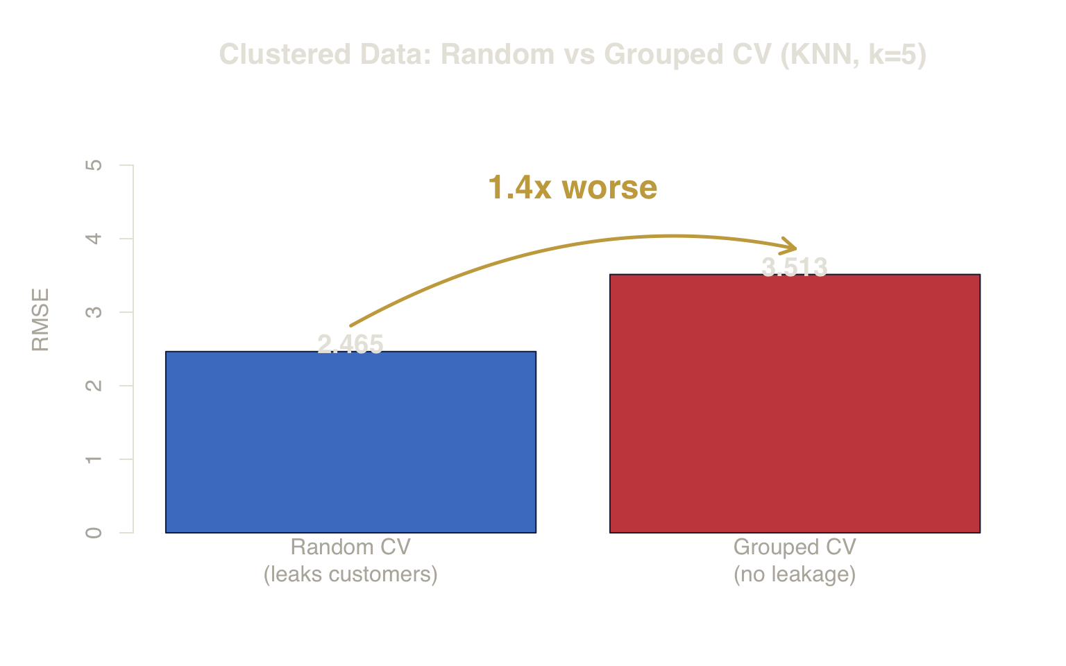
Figure 6. Clustered Data Bias. Random CV reports an artificially low RMSE by leaking customer identities between folds. Grouped CV reveals the true error for new customers.

Random CV RMSE: 2.465 ± 0.031 — artificially low.

Grouped CV RMSE: 3.513 ± 0.213 — realistic.

The gap exists because random CV lets the model access the unobserved intercept (\(\sigma_\alpha\)) through same-customer leakage.

Deployment Insight

If you want to predict how your model works for new individuals, you must validate on new individuals. Any data from the test population that leaks into training will inflate your confidence.

Why the Intercept Leaks

The plot below shows the first 10 customers. Each color is a different customer. The dashed horizontal lines mark each customer’s mean \(y\). Notice the wide vertical spread: some customers sit near \(y \approx 0\), others near \(y \approx 12\). This between-customer variation (\(\sigma_\alpha = 3\)) dwarfs the within-customer scatter (\(\sigma_\varepsilon = 1\)) — and it is exactly what leaks through same-customer rows in random CV.

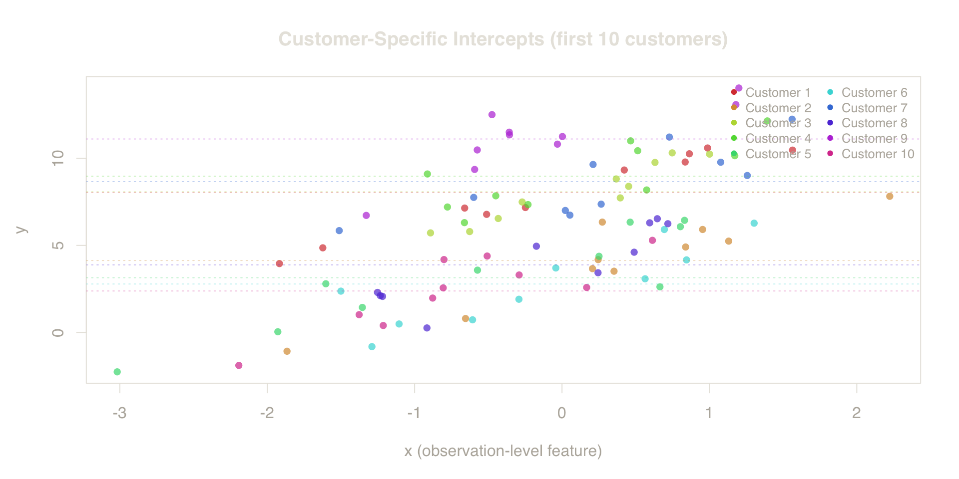
Figure 7. Latent Intercepts. Each color represents a different customer. The wide horizontal spread marks the unobserved heterogeneity that leaks when rows are shuffled randomly.

When random CV scatters these rows across folds, KNN finds same-customer neighbors — rows with identical customer-level features and the same \(\alpha_i\). The model conditions on partial realizations of each customer’s group-level effect, producing predictions that reflect within-customer noise rather than true deployment-level uncertainty. For a truly new customer — one whose \(\alpha_i\) is unknown and whose exact feature combination is absent from training — this conditioning disappears, and the RMSE rises to reflect the between-customer variance that was hidden all along.

Fold-Level Error Distribution

As with the time series, the fold-level view exposes variance differences that point estimates conceal.

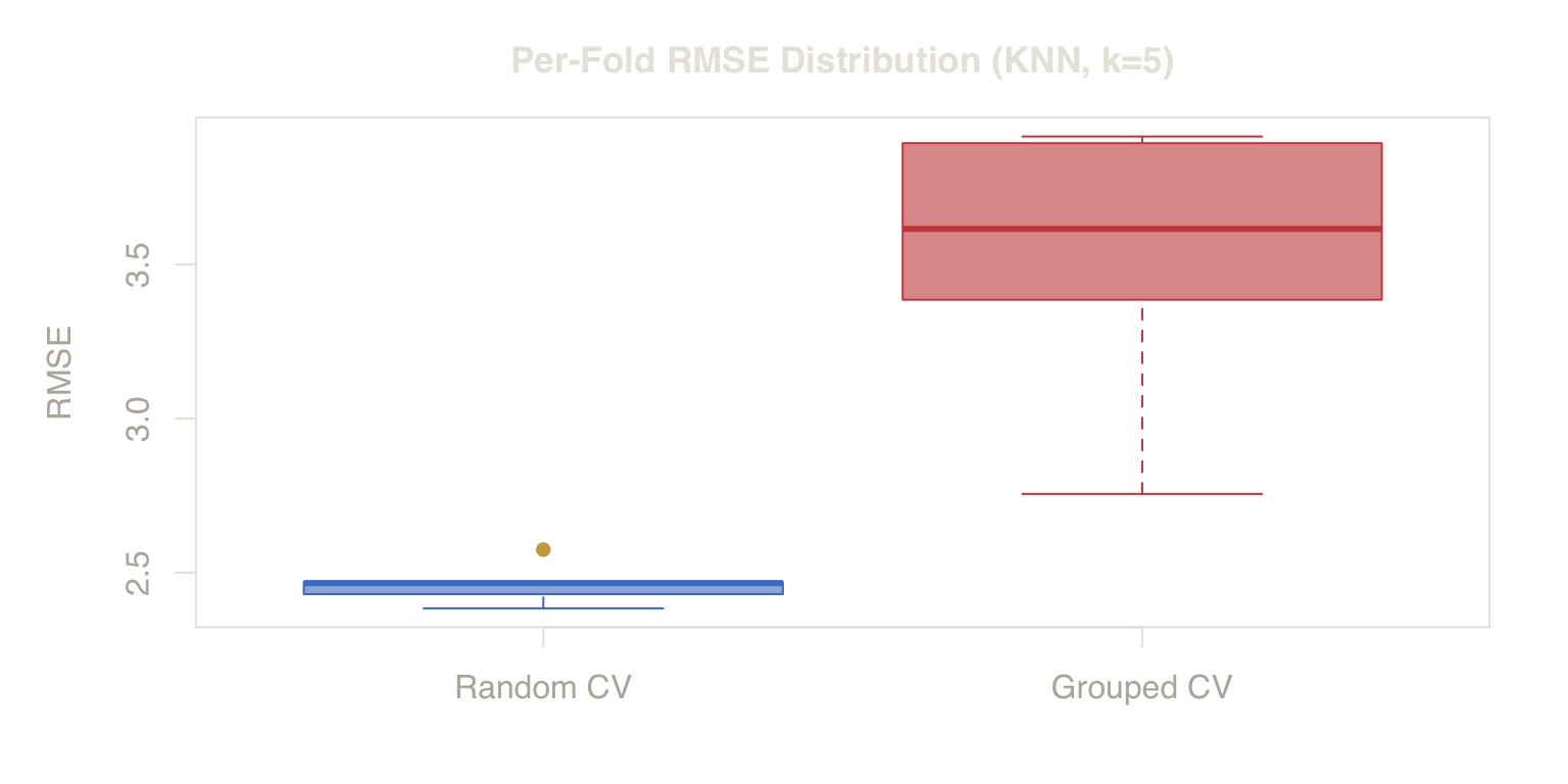
Figure 8. Error Stability vs Reality. Random CV folds cluster tightly around a biased signal. Grouped CV shows higher variance, reflecting the real challenge of predicting unseen clusters.

The random CV folds cluster in a narrow band — every fold sees the same leaked signal, producing artificially stable (and low) error. The grouped CV folds are both higher and more spread, reflecting the genuine unpredictability of unseen customers.

When Does Leakage Matter? The Model Contrast

A critical nuance: not every model exploits the leakage. A simple linear regression fits global coefficients — one intercept, one slope per feature. It cannot condition on customer-specific patterns regardless of how you split the data. KNN, by contrast, is flexible enough to borrow from same-customer neighbors.

To make this concrete, we re-run both CV strategies using lm instead of KNN:

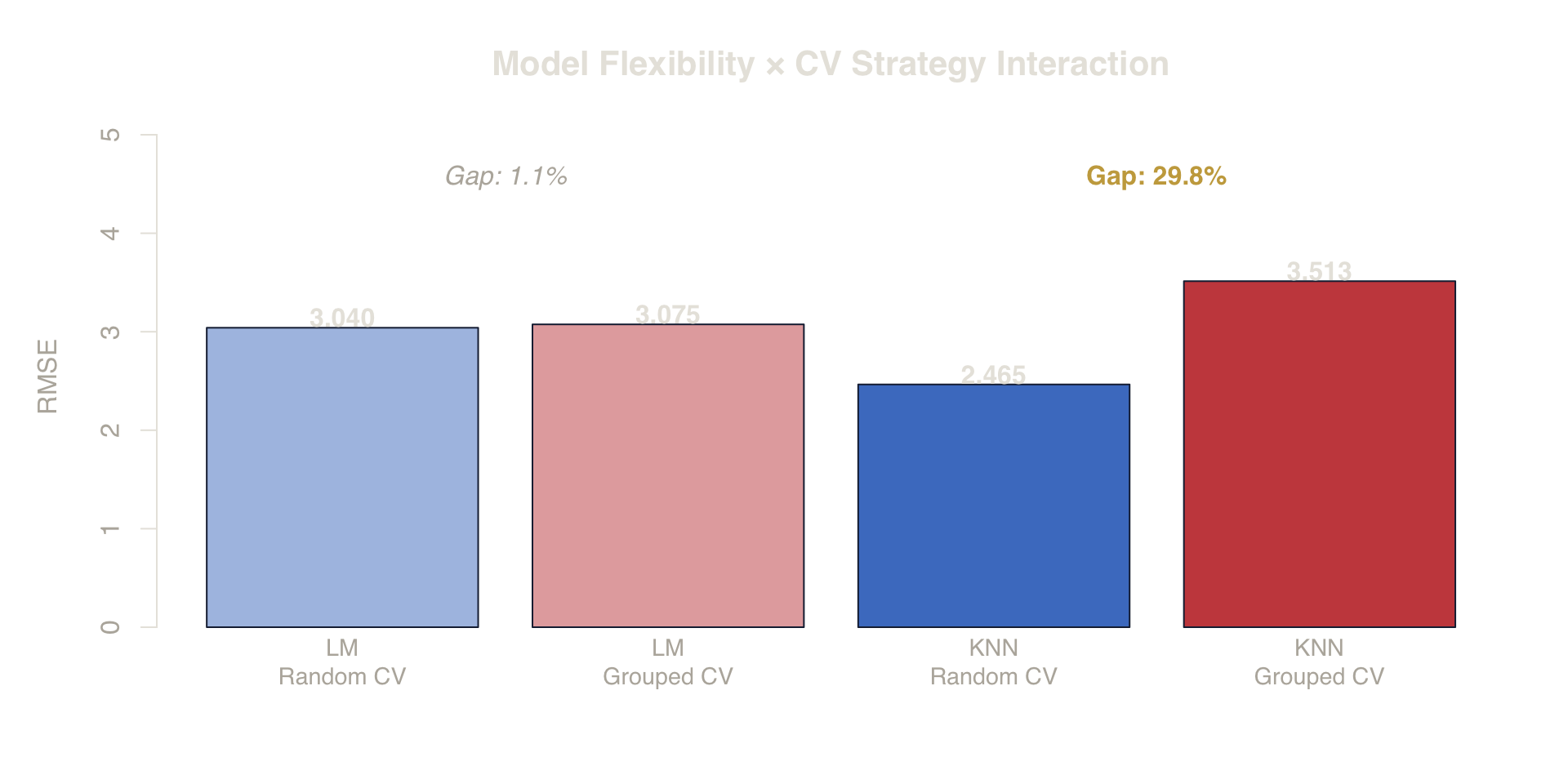
Figure 9. Model Flexibility × CV Interaction. Linear models (LM) are less sensitive to leakage because they can’t isolate group effects. KNN ‘borrows’ the leaked signal, magnifying the evaluation failure.

The linear model shows near-zero gap between random and grouped CV — the same data, the same split, but a different model. KNN shows a large gap.

Deployment Insight

Leakage is a “hidden” signal. Flexible models (trees, KNN, deep learning) are excellent at finding and exploiting that signal. If your evaluation is biased, the most “flexible” model will appear to be the best, while actually being the most overfit to the leakage.

More broadly, model classes differ systematically in their sensitivity to leaked structure:

Model Class	Leakage Sensitivity	Mechanism
Global parametric (LM)	Low	Fits global parameters; cannot condition on group-level signals
Regularized linear (Ridge, Lasso)	Low–moderate	Regularization limits exploitation, but many features can still leak
Tree ensembles (RF, GBM)	High	Partitions feature space; can isolate group-specific splits if group-correlated features exist
Instance-based (KNN)	Very high	Directly borrows from same-group neighbors

Formal Variance Decomposition

The leakage mechanism can be stated formally. Conditional on covariates, the residual variance of \(y\) decomposes as:

Equation 1: Variance Decomposition \[ \text{Var}(y \mid x) = \sigma_\alpha^2 + \sigma_\varepsilon^2 \]

where \(\sigma_\alpha^2 = 9\) is the between-customer variance and \(\sigma_\varepsilon^2 = 1\) is the within-customer noise. The conditional signal-to-noise ratio is \(\sigma_\alpha^2 / \sigma_\varepsilon^2 = 9\).

When random CV includes same-customer rows in training, a flexible model can condition on partial realizations of \(\alpha_i\). The nearest neighbors share the same \(\alpha_i\), so the predictive variance is reduced toward the within-group noise variance \(\sigma_\varepsilon^2\), depending on the extent of same-group overlap. The model appears to explain a large fraction of the variance that it will not be able to access for new customers.

Grouped CV eliminates this conditioning. The model must predict \(y\) without any information about \(\alpha_i\), so the irreducible error includes the full \(\sigma_\alpha^2 + \sigma_\varepsilon^2\). The RMSE transitions from \(\approx \sigma_\varepsilon\) under leakage to \(\approx \sqrt{\sigma_\alpha^2 + \sigma_\varepsilon^2}\) under honest evaluation — a shift fully predicted by the variance decomposition.

This dependence can be approximated analytically. Let \(\pi\) denote the fraction of test-set observations whose group is also present in training (the leakage proportion). Under squared-error loss and approximately balanced group sizes, the expected CV risk scales as:

Equation 2: Expected CV Risk with Leakage \[ \mathbb{E}[\widehat{R}_{CV}] \approx \sigma_\varepsilon^2 + (1 - \pi)\,\sigma_\alpha^2 \]

When \(\pi \to 1\) (random CV with many same-group rows in training), the second term vanishes and CV reports only within-group noise. When \(\pi = 0\) (grouped CV), the full between-group variance is included. The optimism bias thus scales directly with leakage density.

Deployment Insight

This analytical approximation highlights the core problem: random CV (where \(\pi \to 1\)) effectively removes the between-group variance (\(\sigma_\alpha^2\)) from the estimated risk, leading to an optimistic error estimate. Grouped CV (where \(\pi = 0\)) correctly includes this variance, providing a realistic assessment for new groups.

Sensitivity: Bias vs Signal-to-Noise Ratio

The variance decomposition predicts that optimism bias increases with \(\sigma_\alpha / \sigma_\varepsilon\). The table below verifies this empirically by re-running the KNN simulation across a range of signal-to-noise ratios while holding all else constant.

Optimism Bias Scales with Between-Group Variance (B = 50 replications)

σ_α	σ_α/σ_ε	Random CV	Grouped CV	Bias (%)
0.0	0.0	1.135 ± 0.028	1.134 ± 0.030	-0.1%
0.5	0.5	1.220 ± 0.033	1.293 ± 0.043	5.7%
1.0	1.0	1.429 ± 0.053	1.637 ± 0.080	12.7%
2.0	2.0	2.067 ± 0.122	2.624 ± 0.179	21.2%
3.0	3.0	2.896 ± 0.177	3.831 ± 0.281	24.4%
5.0	5.0	4.413 ± 0.387	5.965 ± 0.546	26.0%

As predicted by the variance decomposition: when \(\sigma_\alpha = 0\) (no group structure), the bias vanishes — random and grouped CV agree. As \(\sigma_\alpha / \sigma_\varepsilon\) increases, the gap widens broadly across all conditions (minor non-monotonicity in the final row is attributable to Monte Carlo variability). Averaging over \(B = 50\) replications eliminates most sampling noise, confirming that the optimism bias is a direct, predictable function of the unobserved heterogeneity magnitude.

The Structural Fix: Mixed-Effects Modeling

It is important to distinguish two separate problems:

• Evaluation failure: The CV split produces a biased error estimate. Fix: grouped CV.
• Modeling failure: The model does not represent group-level heterogeneity. Fix: mixed-effects model.

Grouped CV corrects the evaluation. It does not improve the model. The analysis above shows that KNN diagnoses the leakage through grouped CV but does not fix the underlying representation gap. A mixed-effects model addresses the root cause by estimating \(\alpha_i\) as random effects:

Equation 3: Mixed-Effects Model for Clustered Data \[ y_{ij} = \underbrace{(\beta_0 + \alpha_i)}_{\text{random intercept}} + \beta_1 f_{1i} + \beta_2 f_{2i} + \beta_3 x_{ij} + \varepsilon_{ij} \]

The lmer() function from lme4 (Bates et al., 2015) fits this model directly, partitioning the variance between the customer-level random effects and observation-level noise.

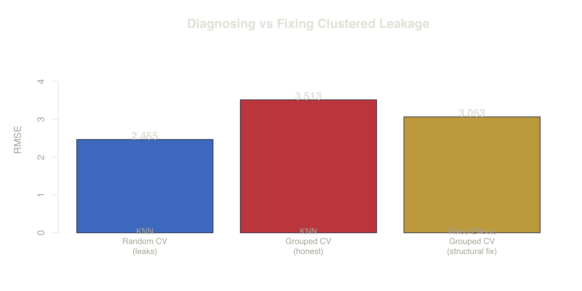
Figure 10. Diagnosing vs Fixing. Grouped CV (red) honestly diagnoses the leakage in KNN. Mixed-effects models (gold) structurally fix the model to account for group heterogeneity.

Three key observations:

1. KNN Random CV (blue) — the optimistic estimate with leakage.
2. KNN Grouped CV (red) — the honest estimate, revealing the full between-customer error.
3. Mixed-Effects Grouped CV (gold) — the RMSE when the model structurally accounts for customer heterogeneity. By estimating \(\alpha_i\) as random effects, the model explicitly partitions between- and within-customer variance. For new customers (where re.form = NA drops the random effect), prediction relies on fixed effects only. For existing customers with repeated measures, the model can use best linear unbiased predictors (BLUPs) of \(\alpha_i\) to improve accuracy.

The mixed-effects model does not eliminate the between-customer error for unseen customers — it cannot predict \(\alpha_i\) without data — but it correctly separates the explainable variation from the irreducible.

Deployment Insight

A structural fix is better than an evaluation correction alone. Mixed-effects models and temporal feature engineering address the root cause of the failure, making your model inherently more robust to the non-IID nature of the data.

4. The Exchangeability Assumption

The Exchangeability Requirement for Valid Cross-Validation

\(k\)-fold cross-validation provides a consistent estimate of generalization error when observations are exchangeable — i.e., any permutation of \((x_1, y_1), \ldots, (x_n, y_n)\) has the same joint distribution.

Exchangeability is a sufficient condition. Under certain weak dependence structures (e.g., \(\alpha\)-mixing or \(\beta\)-mixing processes), CV can still be asymptotically valid with appropriate variance corrections (Racine, 2000). Under stationary mixing processes, blocked CV converges to the same risk as horizon-\(h\) test error as \(n \to \infty\). However, the violations below are not weak:

• Temporal dependence: \(P(y_t \mid x_t)\) depends on \(t\), so shuffling destroys the time structure. Random CV estimates \(\mathcal{R}_{mix}\) under \(P_{mix}\), not \(\mathcal{R}_{deploy}\) under \(P_{future}\).
• Grouped dependence: Observations within group \(g\) share latent variables \(\alpha_g\), so splitting within groups allows flexible models to condition on partial realizations of \(\alpha_g\).

In both cases, random CV estimates the expected loss under the reshuffled distribution, not under deployment-realistic splits. The result is anti-conservative (optimistic) error estimates whose magnitude depends on both the severity of the structural violation and the flexibility of the model.

A note on severity and bias magnitude

The optimism bias is not binary. It scales with:

1. Magnitude of structural violation — a mild drift produces less bias than a regime flip (cf. Section 2 vs 2b).
2. Model flexibility — global parametric models may show near-zero bias under the same split where instance-based models show large bias (cf. Section 3, Model Contrast).
3. Deployment horizon — if the deployment target is only slightly ahead of training (short horizon), even drifting data may show small bias.

CV is not “always wrong” under non-IID data. The relevant question is always: how large is the mismatch between \(P_{mix}\) and \(P_{future}\), and can the model exploit the leaked structure?

Decision Tree

Before choosing a validation strategy, ask: “Can I shuffle the rows without changing the problem?” If the answer is no, standard CV targets the wrong error. The table below maps common data structures to the correct validation approach (Roberts et al., 2017).

Data Structure	IID Valid?	Correct Method	Rationale
Independent rows, no time	Yes	Random \(k\)-fold CV	Standard regime
Time-ordered, predict future	No	Time-blocked split or expanding window	Future cannot leak into training
Repeated measures per subject	No	Grouped CV (leave-group-out)	Intra-subject correlation inflates fit
Spatial data (e.g., neighboring plots)	No	Spatial blocking or buffered CV	Nearby points are autocorrelated
Time + clusters (panel data)	No	Time-blocked with group awareness	Both dimensions must be respected

5. Summary

The table below collects every RMSE from both experiments. In each case, the naive method (Random CV) produces a lower RMSE than the correct method — not because the model is better, but because the evaluation admits structural information that will not exist at deployment time.

Optimism Bias: Same Model, Different Split

Scenario	Method	RMSE	SE	Optimism Bias	Verdict
Regime Shift	Random CV	2.228	± 0.023	44.9%	Optimistic
Regime Shift	Blocked Split	4.044	—	—	Realistic
Gradual Drift	Random CV	1.073	± 0.013	7.3%	Optimistic
Gradual Drift	Blocked Split	1.157	—	—	Realistic
Clustered (KNN)	Random CV	2.465	± 0.031	29.8%	Optimistic
Clustered (KNN)	Grouped CV	3.513	± 0.213	—	Realistic

The optimism bias column quantifies \(\frac{RMSE_{\text{proper}} - RMSE_{\text{naive}}}{RMSE_{\text{proper}}}\) — the fraction of the true error that random CV hides.

Structural Correction: Same Split, Different Model

Model	CV Strategy	RMSE	Improvement
KNN (k=5)	Grouped CV	3.513	—
Mixed-Effects (lmer)	Grouped CV	3.063	12.8%

Random CV assumes IID data.

Time shifts and clustered structure violate IID.

When structure is ignored, CV underestimates true error.

Proper blocking or grouping reveals realistic performance.

6. Key Takeaways

1. Random CV is not universally safe. It targets the right error only when exchangeability holds. If you have not verified exchangeability, your error estimate may be estimating the wrong quantity.

2. Temporal data requires time-aware splits. Train on the past, test on the future. Shuffling time series data conflates training and deployment distributions.

3. Model flexibility magnifies evaluation failure. The more flexible your model (e.g., KNN, RF, GBM), the more aggressively it will exploit leaked structure. Honest evaluation is most critical for your most powerful models.

Final Takeaway

The goal of validation is not to get the lowest RMSE. The goal is to get the most accurate estimate of the RMSE you will see in the real world. If you can’t shuffle your data without breaking its meaning, don’t shuffle it for your validation.

4. The gap between naive and proper validation quantifies your deployment risk. The larger the gap, the more the deployed model will underperform relative to internal evaluation estimates.

5. Use the deployment test for every split: “Could this train/test partition actually occur in production?” If the test set contains data the model would never have at prediction time, the error estimate is conditioned on a distribution that differs from deployment.

6. Consider the model, not just the split. Leakage magnitude depends on model flexibility. A global linear model may show no gap under the same split where KNN or random forest shows a large one. The split strategy and the model class interact.

7. Limitations

The simulations above are designed to isolate specific failure modes of random CV under controlled conditions. Several scope boundaries should be noted:

• Low-dimensional feature spaces. All simulations use 1–3 features. In high-dimensional settings, KNN’s ability to find same-customer neighbors may be diluted by irrelevant features, reducing the leakage magnitude relative to what is shown here.
• Fixed hyperparameters. KNN uses \(k = 5\) throughout. The leakage mechanism operates at any \(k\), but the bias magnitude varies: smaller \(k\) amplifies same-customer borrowing, while larger \(k\) dilutes it.
• Gaussian, homoskedastic noise. All error terms are \(\mathcal{N}(0, 1)\). Heavy-tailed or heteroskedastic noise could alter both the variance decomposition and the relative magnitude of optimism bias.
• Balanced group sizes. All customers have exactly 10 observations. The \(\pi\)-based approximation assumes approximately balanced groups; unbalanced designs would require a weighted formulation.
• Single-seed main simulations. The regime-shift, drift, and clustered experiments each use a single random seed. The sensitivity table, by contrast, averages over \(B = 50\) replications per condition to ensure robustness.

These constraints do not affect the qualitative conclusions — the mechanisms are general — but quantitative magnitudes (e.g., “2.8x worse”) are specific to the simulation parameters chosen.

References

• Arlot, S., & Celisse, A. (2010). A survey of cross-validation procedures for model selection. Statistics Surveys, 4, 40–79.
• Bergmeir, C., & Benítez, J. M. (2012). On the use of cross-validation for time series predictor evaluation. Information Sciences, 191, 192–213.
• Roberts, D. R., et al. (2017). Cross-validation strategies for data with temporal, spatial, hierarchical, or phylogenetic structure. Ecography, 40(8), 913–929.
• Hastie, T., Tibshirani, R., & Friedman, J. (2009). The Elements of Statistical Learning. Springer. Chapter 7.
• Bates, D., Mächler, M., Bolker, B., & Walker, S. (2015). Fitting Linear Mixed-Effects Models Using lme4. Journal of Statistical Software, 67(1), 1–48.
• Tashman, L. J. (2000). Out-of-sample tests of forecasting accuracy: an analysis and review. International Journal of Forecasting, 16(4), 437–450.
• Racine, J. (2000). Consistent cross-validatory model-selection for dependent data: hv-block cross-validation. Journal of Econometrics, 99(1), 39–61.

Generated with R 4.5.1 and caret 7.0.1 · marcelokatogui.com